- Published on
Dimensional Modeling - Part 1: Basic Fact Table Techniques
- Authors

- Name
- Mai Khoi TIEU
- @tieukhoimai
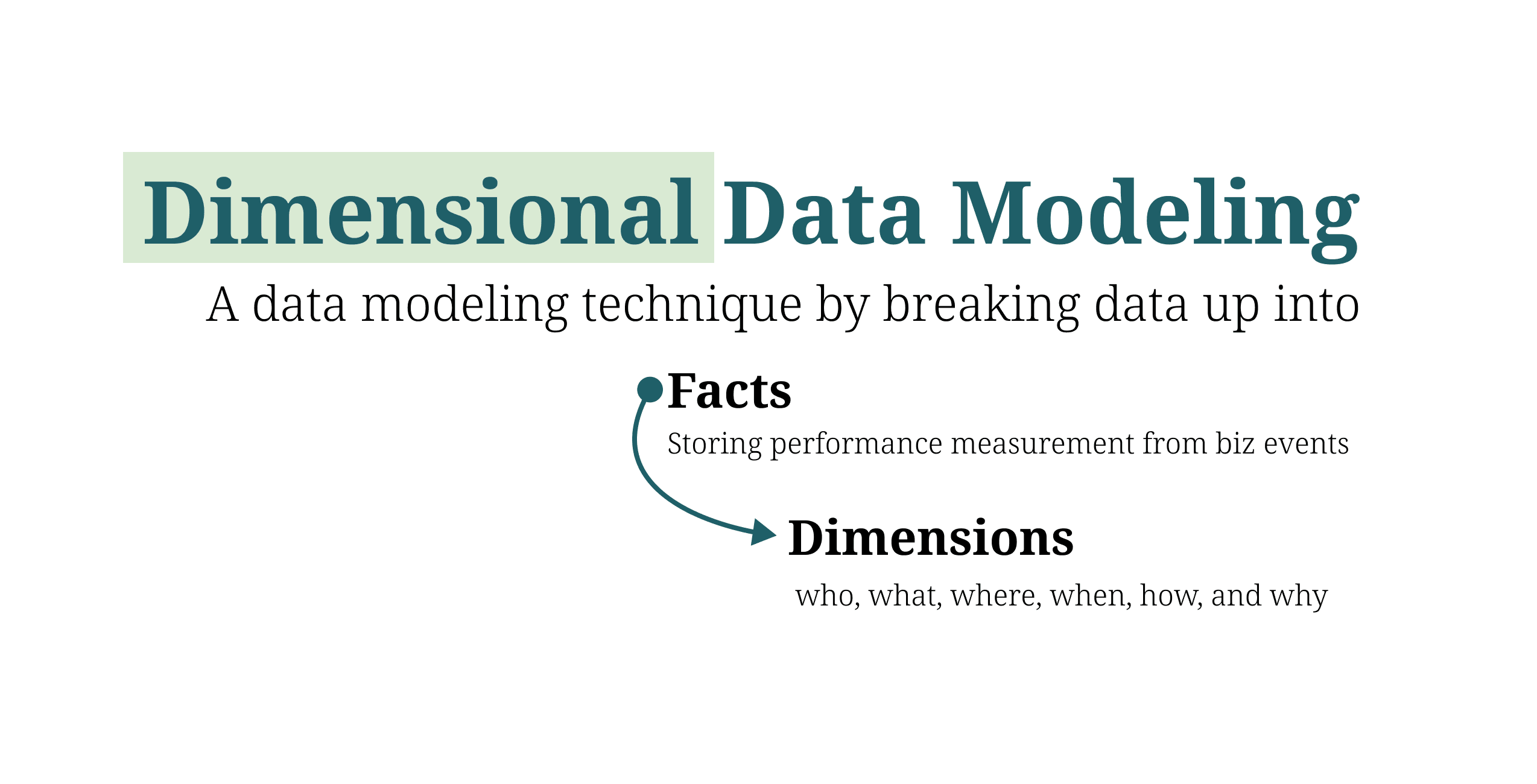
Table of Contents
1. Introduction
In this article, I will introduce the concept of the Basic Fact table in Dimensional data modeling. This technique was first published in The Data Warehouse Toolkit: The Definitive Guide to Dimensional Modeling in 1996. To understand this technique, we will explore the different types of data modeling, including the relational data model, Entity Relationship model, Hierarchical data model, Object-Oriented model, and Dimensional data model. The Dimensional data model is composed of a fact table and dimension tables. This article will also recap some fundamental knowledge, including the star and snowflake schemas, which are common approaches to Dimensional data modeling. Additionally, we will explain the differences between these schemas by exploring the concepts of normalization.

Fig 1. Data modeling overview
2. What is data modeling
Data modeling is the process of creating a conceptual representation of data and its relationships, which helps us understand how data is stored, accessed, updated, and queried within the database. The output of that process is a formal description of the data that has been modeled, which is called a data model. A data model can be compared to a roadmap, an architect's blueprint, or any formal diagram that facilitates a deeper understanding of what is being designed [1]

Fig 2. Three level of data modeling
There are three different levels of data modeling: conceptual data models, logical data models, and physical data models.
- A conceptual data model consists of highly abstract levels of data elements called entities and relationships between entities. It presents a high-level overview of the database system through a visual representation of the entities it contains and their relationships to one another. The conceptual model provides the basis for the logical data model.
- A logical data model builds on the conceptual model by providing a more detailed overview of the entities in their respective relationships. It identifies the attributes of each entity, defines the primary keys, and specifies the foreign keys. The logical data model serves as an intermediary between the high-level conceptual model and the physical implementation. It describes how the data will be organized in the database and provides a blueprint for building the physical database.
- A physical data model is used to create the schema of the database, which is then implemented in the database management system. The physical data model defines the structure of the database, including the data types, constraints, and attributes. It specifies how the data will be stored in the specific database management system being used.
In conclusion, a conceptual data model is a high-level view of the database that is used to communicate with stakeholders about the requirements of the database. The conceptual data model can then be used to create a logical data model, which is a more detailed view of the database that includes the relationships between entities, and the constraints and rules that apply to the data. Finally, the logical data model can be used to create a physical data model, which is the actual database schema that is implemented in a database management system.
3. Types of data modeling

Fig 3. Common types of data modeling
3.1. Relational data model
The relational data model is based on the idea that data is stored in tables with columns that correspond to attributes and rows that correspond to individual records. The model is named "relational" because it emphasizes the relationships between tables, which are established through the use of primary and foreign keys.

Fig 4: Relational data model [2]
3.2. Entity Relationship model
The entity-relationship model, on the other hand, is designed to represent complex relationships between entities, such as one-to-one, one-to-many, and many-to-many relationships. It uses symbols such as diamonds and arrows to represent these relationships in a visual way that is easy to understand.
The ER model is based on the concept of a real-world entity, such as a person, place, or thing, that has attributes that describe it, and relationships with other entities.

Fig 5. Entity Relationship diagram (Refer the conventions for diagramming in [3]
For example, in a university database, a student is an entity, with attributes like ID, name, and group id, and relationships with other entities like teacher, subject, and other students (ex: same group).
3.3. Hierarchical data model
The hierarchical data model is typically used to represent data that has a strict parent-child relationship, such as the organization of a company or the structure of a file system. It is often used in mainframe and legacy systems.

Fig 6. Hierarchical data model)
The major disadvantage of hierarchical databases is their inflexible nature. The one-to-many structure is not ideal for complex structures as it cannot describe relationships in which each child node has multiple parents nodes. [4]
3.4. Object oriented model
The object-oriented model is based on the idea of objects, which are self-contained units of code that encapsulate data and behavior. The model is designed to be flexible and adaptable, allowing developers to create new types of objects as needed.
Object-oriented data model is a conceptual data model that is designed to represent real-world objects and their relationships to one another. It is not inherently tied to any specific database technology, but it can be implemented using a variety of different database management systems. There are some NoSQL databases especially document-based, are particularly well-suited to storing and querying complex, nested data structures that are common in object-oriented data modeling. that are designed to work with object-oriented data models. These databases provide features such as document storage, indexing, and querying, and allow for the storage of complex objects with nested structures. NoSQL databases.

Fig 7. Object Oriented and Relational data mode [5]
MongoDB is one of the popular NoSQL databases that is particularly well-suited to storing and querying complex, nested data structures that are common in object-oriented data modeling. It is a document-based database that allows data to be stored in flexible, JSON-like documents, making it an ideal choice for developers who work with object-oriented data models. MongoDB provides features such as document storage, indexing, and querying, and allows for the storage of complex objects with nested structures.
MongoDB also provides support for horizontal scaling, allowing it to handle large volumes of data with ease. It uses a sharding technique to distribute data across multiple nodes in a cluster, which enables it to scale horizontally without sacrificing performance. Additionally, MongoDB supports dynamic schema, which means that data can be added to the database without the need for pre-defined schema or table structures.
3.5. Dimensional data model
The dimensional data model is specifically designed for data warehousing and business intelligence applications. It is optimized for fast queries and analysis by structuring data into "facts" (measures) and "dimensions" (attributes), which can be easily analyzed using OLAP tools.
4. Normalization
Normalization is the process of structuring tables to resolve anomalies such as the insertion anomaly, the update anomaly and the deletion anomaly. There are three common levels of data normalization that are used to resolve these anomalies.

Fig 9. Overview of Normalization
- First Normal Form (1NF) - This level focuses on data atomicity by ensuring that multiple fields are not used to store similar data in a single table.
- Second Normal Form (2NF) - This level fixes relationships built on functional dependencies by ensuring that records depend only on a table's primary key.
- Third Normal Form (3NF) - This level resolves transitive dependencies by ensuring that values in a record that are not part of that record's key do not belong in the table.
Each level builds on the previous one and helps to ensure that the database is free from redundancy and anomalies, which can improve its performance and maintainability. Refer a process of normalizing an example table in [6]
5. Star and Snowflake schema

Fig 10. Star and Snowflake Schema [7]
Star and snowflake schemas are two common dimensional data models used in dimensional modeling approach.
A star schema consists of a central fact table connected to multiple dimension tables, forming a star shape. The dimension tables contain descriptive attributes related to the fact table's measures. In contrast, a snowflake schema has normalized dimension tables with hierarchical relationships, leading to a more complex structure. Both schemas have their advantages and disadvantages, with the choice often depending on the specific requirements of the system and the trade off between query performance and storage efficiency.

Fig 11. Difference between star and snowflake schema
6. Types of fact tables
A fact table is a fundamental table in a dimensional data model that stores the numerical measurements or facts of a business process. These facts describe a specific event or transaction, such as a sale, a shipment, or a website click. Fact tables typically have one or more foreign keys that link to dimension tables, which provide descriptive information about the event or transaction.

Fig 12. Types of fact tables
There are three types of facts:
- Additive facts are measures that can be aggregated or summed across any of the dimensions associated with the fact table. Examples include sales revenue, units sold, or profit.
- Semi-additive facts are measures that can be aggregated or summed across some dimensions, but not all. These types of facts are typically used in periodic snapshot fact tables that capture the state of a business process at a specific point in time. Examples include account balances or inventory levels.
- Non-additive facts are measures that cannot be aggregated or summed across any dimension. Instead, they represent calculations that involve complex formulas or functions. Examples include margins, ratios, percentages, or calculated averages.
There are several types of fact tables, including:
- Transaction fact tables, where each row corresponds to a measurement event at a point in space and time.
- Periodic fact tables, where each row summarizes many measurement events occurring over a standard period, such as a day, a week, or a month. The grain is the period.
- Accumulating snapshot fact tables, where each row summarizes the measurement events occurring at predictable steps between the beginning and the end of a process.
- Factless fact tables, which are used to model the absence or occurrence of certain events or conditions. A factless fact table contains all the possibilities of events that might happen, and an activity table contains the events that did happen.
The choice of a fact table type depends on the nature of the business process and the analytical requirements of the system. Fact tables can help answer many different types of questions, from simple counts and averages to complex correlations and predictions.
6.1. Transaction Fact Tables
The transaction grain represents a measurement event defined at a particular instant. A row in a transaction fact table corresponds to a measurement event at a point in space and time.
For example, each time we make a transaction action by pressing PLACE ORDER, it will INSERT a record into this fact table.

Fig 13. Transaction Fact Tables
Characteristics of transaction fact table
- Lowest level of granularity
- Mostly additive fact
- Largest database size
- Highly need for aggregate tables
6.2. Periodic Fact Tables
A periodic fact table or periodic fact entity stores one row for a group of transactions that happen over a period of time. The source data of the periodic snapshots fact table is data from a transaction fact table where choosing a period to get the output.
For example, the periodic fact table will be INSERT a new row aggregated in month level (one row per time period)

Fig 14. Periodic Fact Tables
Characteristics of periodic fact table
- End-of-period granularity
- Be stored at a high aggregated level
- Related to periodic activities
- Mostly semi-additive fact
6.3. Accumulating snapshot fact tables
The accumulating snapshots fact table describes the activity of a business process that has a clear beginning and end. This type of fact table, therefore, has multiple date columns to represent milestones in the process.
For example: when we PLACE ORDER, it will INSERT a new row to record the Order ID and Order Placed Date. Until this order was paid/shipped out/received/completed, or we can say that when a milestone is reached for a particular activity this will UPDATE on this fact table.

Fig 15. Accumulating snapshot fact tables
Characteristics of Accumulating snapshot fact table
- One row for the entire lifetime of an event
- UPDATE when a milestone is reached for a particular activity
- Related to activities which have a definite lifetime
6.4. Factless fact tables
Factless fact tables can also be used to analyze what didn’t happen. These queries always have two parts: a factless coverage table that contains all the possibilities of events that might happen and an activity table that contains the events that did happen. When the activity is subtracted from the coverage, the result is the set of events that did not happen. [8]
A factless fact table doesn't include any measure columns. It contains only dimension keys.
For example: To answer the question that “What Products were on promotion but did not sell?. We will have list of products sold (Sell), illustrated as Fig 16 and list of products that were on promotion on a given day which called factless fact table (Promotion), illustrated as Fig 17.

Fig 16: Fact Sales (Sell) - List of products sold

Fig 17: Fact Promotion (Promotion) - List of products that were on promotion on a given day
Therefore, Product were on promotion but did not sell
= Promotion - (Promotion ∩ Sell)
= Promotion - Sell

Fig 18: Venn Diagram to describe factless fact table
7. Reference
- IBM. (n.d.). Data modeling. Retrieved April 2, 2023.
- Varatharajan, S. (2022, January 19). Relational Data Model in DBMS: Concepts, Constraints, Examples. Guru99.
- Lucidchart. (n.d.). ER Diagrams. Retrieved April 3, 2023.
- Heavy AI. (n.d.). Hierarchical Database. Heavy Technical Glossary. Retrieved April 7, 2023.
- MongoDB. "What is an Object-Oriented Database?" MongoDB, Accessed 2 Apr. 2023.
- Microsoft. "Database Normalization Description." Microsoft Office Support, Microsoft, 22 Aug. 2020
- PhoenixNAP. (n.d.). Star schema vs snowflake schema: What's the difference? Retrieved April 5, 2023
- Kimball Group. (n.d.). Factless Fact Table. Retrieved April 7, 2023