Gaussian Naive Bayes

This article is based on my personal lecture notes from my studies at Machine Learning for Data Science 2023/2024 course: Bayesian Learning. The content reflects my understanding and interpretation of the course material.

Objective

Given a data point x, what is the probability of x belonging to some class c?

We have C class and need to find which group of $x$ , instead of finding exactly the label, given a data point x, we find the probability of x belonging to some class c or find $P(y=c|x)$ or $P(c|x)$

c = \argmax_c P(c|X)

We define the class of each point by choosing the class c with the highest probability

Bayes’ theorem

P(A|B) = \frac{P(B|A)P(A)}{P(B)}

Naive Bayes Classifier formula

P(c|x) = \frac{p(x|c)P(c)}{p(x)} = \frac{p(x|c)P(c)}{\sum_{c}p(x|c)p(c)}

Posterior = \frac{Likelihood \times Prior}{Evidence}

where

$x$ consists $x_{ij}$ with $i=\overline{1,n}$ with $n$ = observation and $j=\overline{1,n}$ with $k$ is the number of features
$P(c|x)$ is Posterior Probability
$p(x|c)$ is Likelihood of feature $x_j$ given that their class is T
$P(c)$ is Prior Probability
$P(x)$ is Marginal Probability or called Evidence

We have

c = \argmax_c P(c|X)=\argmax_c \frac{p(x|c)P(c)}{p(x)} = \argmax_c p(x|c)P(c)

Implementation

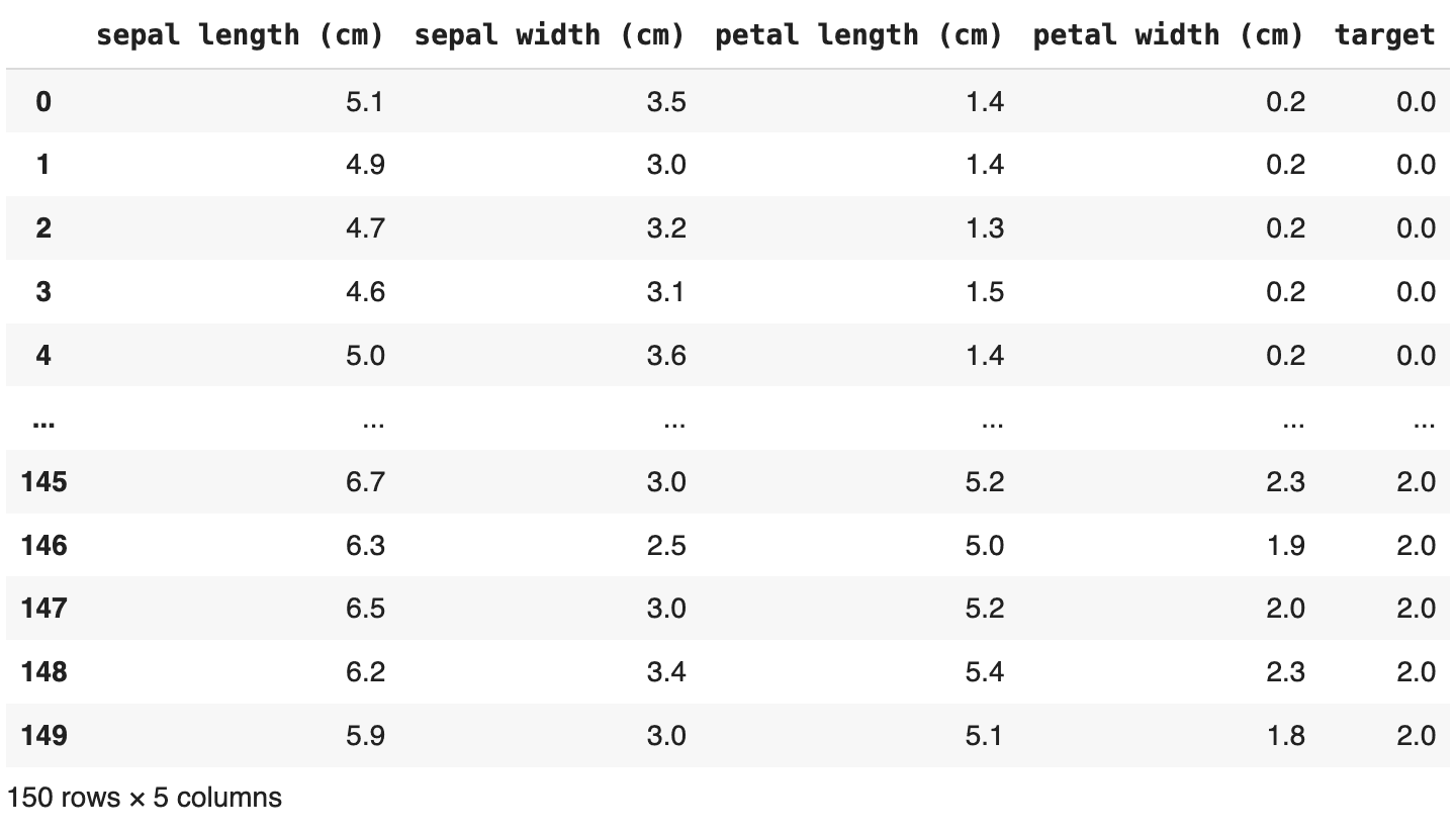
We choose Iris as a dataset.

from sklearn.datasets import load_iris
import matplotlib.pyplot as plt

x, y = load_iris( return_X_y=True )

There are

3 classes $c_1, c_2, c_3$
150 observations with 4 features $x_1, x_2, x_3, x_4$

Likelihood of each feature per class

Computing $P(x|c)$ depends on the type of data. There are three commonly used types: Gaussian Naive Bayes, Multinomial Naive Bayes, and Bernoulli Naive Baye

We will consider the Gaussian distribution, with two common distributions: the univariate normal distribution (or Gaussian density) and the multivariate normal distribution (or multivariate density).

Univariate normal distribution or Gaussian density

p(x) = \frac{1}{\sqrt{2\pi \sigma^2}}e^{(-\frac{(x-\mu)^2}{2\sigma^2})}

This distribution is described by two parameters: the mean $\mu$ and the variance $\sigma^2$ .

The value of $\mu$ can be any real number, indicating the location of the peak, where the probability density function reaches its highest value.
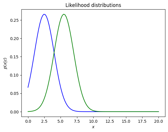
Example: Plot the gaussian distributions (likelihood) with the $\mu_1$ < $\mu_2$ and same variance

import numpy as np
import matplotlib.pyplot as plt
from scipy.stats import norm

# Generate the functions' domain
x = np.linspace(0,20,100)

# Define two gaussian distributions

p1 = norm.pdf(x, 2.5, 1.5)
p2 = norm.pdf(x, 5.5, 1.5)

# Plot the gaussian distributions (likelihood)
plt.plot( x, p1, 'b')
plt.plot( x, p2, 'g')
plt.title('Likelihood distributions')
plt.ylabel('$p(x|c)$')
plt.xlabel('$x$')
plt.show()

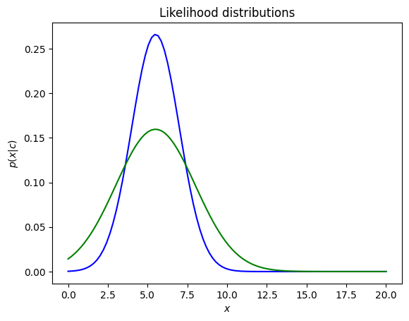
The value of $\sigma^2$ is a positive value, with $\sigma$ representing the spread of this distribution. A large $\sigma$ indicates a wide range of output values, and vice versa.
Example: Plot the gaussian distributions (likelihood) with the $\sigma_1$ < $\sigma_2$ and same variance

import numpy as np
import matplotlib.pyplot as plt
from scipy.stats import norm

# Generate the functions' domain
x = np.linspace(0,20,100)

# Define two gaussian distributions

p1 = norm.pdf(x, 5.5, 1.5)
p2 = norm.pdf(x, 5.5, 2.5)

# Plot the gaussian distributions (likelihood)
plt.plot( x, p1, 'b')
plt.plot( x, p2, 'g')
plt.title('Likelihood distributions')
plt.ylabel('$p(x|c)$')
plt.xlabel('$x$')
plt.show()

Multivariate normal distribution (or multivariate density)

This is the general case of the normal distribution when the variable is multidimensional, assuming it has $d$ dimensions.

p(x) = \frac{1}{(2\pi)^{d/2}|\Sigma|^{1/2}}\exp\left(-\frac{1}{2}(x - \mu)^T \Sigma^{-1} (x - \mu)\right)

where

$x$ is $d$ -component column vector
$\mu \in \mathbb{R}^d$ is $d$ -component mean vector
$\Sigma \in \mathcal{S}^D_{++}$ is $d \times d$ matrix and a positive definite symmetric matrix.

Back to our example with Iris dataset, we compute the likelihood for each sample and each class.

import numpy as np
from scipy.stats import multivariate_normal

# Identify members of each class -> 4 column vector with 150 obs
cl1 = x[ y==0, :]
cl2 = x[ y==1, :]
cl3 = x[ y==2, :]

# Compute the mean (centroid) of each class -> return a 4 row vector
m1 = np.mean(cl1, axis = 0)
m2 = np.mean(cl2, axis = 0)
m3 = np.mean(cl3, axis = 0)

# Compute the covariance matrix for each class -> return a 4x4 matrix (4 features)
C1 = np.cov(cl1.T) # or using C1 = np.cov(cl1, rowvar=False)
C2 = np.cov(cl2.T)
C3 = np.cov(cl3.T)

# compute the likelihood for each sample and each class
lik1 = multivariate_normal.pdf(x, mean=m1, cov=C1)
lik2 = multivariate_normal.pdf(x, mean=m2, cov=C2)
lik3 = multivariate_normal.pdf(x, mean=m3, cov=C3)

Prior Probability

Each value $P(c)$ , where $c = 1, 2, \ldots, C$ , can be determined as the frequency of occurrence of class $c$ in the training data.

# Define the priors
P_c1 = np.size(cl1)/np.size(x) # 1/3
P_c2 = np.size(cl2)/np.size(x) # 1/3
P_c3 = np.size(cl3)/np.size(x) # 1/3

Marginal distribution or Evidence

We compute $p(x)$ in this case of 3 classes

{p(x)} = {\sum_{c=1}^{3}p(x|c)p(c)} = p(x|c_1)p(c_1) + p(x|c_2)p(c_2) + p(x|c_3)p(c_3)

p_x = (lik1 * P_c1) + (lik2 * P_c1) + (lik3 * P_c1)

Posterior Probabilities

P(c|x) = \frac{p(x|c)P(c)}{p(x)}

# Compute posterior probabilities
post1 = (lik1 * P_c1) / p_x # shape = (150,)
post2 = (lik2 * P_c2) / p_x # shape = (150,)
post3 = (lik3 * P_c3) / p_x # shape = (150,)

post = np.vstack((post1,post2,post3)) # shape = (3,150)

Making Prediction

c = \argmax_{c \in \{1, \ldots, C\}}P(c|x)=\argmax_{c \in \{1, \ldots, C\}} \prod_{i=1}^{d} p(x_i|c)p(c)

When $d$ is large and the probabilities are small, the expression on the right-hand side of equation above becomes a very small number, leading to potential numerical inaccuracies during computation. To address this, equation above is often rewritten in an equivalent form by taking the logarithm of the right-hand side

c = \argmax_{c \in \{1, \ldots, C\}}logP(c|x)=\argmax_{c \in \{1, \ldots, C\}} \sum_{i=1}^{d} log(p(x_i|c)) + log(p(c))

In this case, with $d=3$ , the results of the logarithm of the posterior probabilities and the posterior probabilities are equal.

logpost = np.log(post)
prediction = np.argmax(logpost,axis=0)
accuracy = np.sum(prediction == y)/len(y)

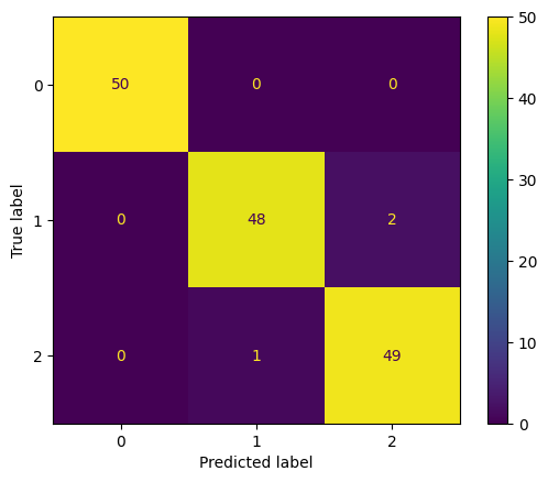
# Classifier accuracy: 98.00%
print('Classifier accuracy: ' + "{0:.2f}".format(accuracy*100) + '%')

# Visualize confusion matrix
from sklearn.metrics import confusion_matrix
cm = confusion_matrix(y,prediction)
from sklearn.metrics import ConfusionMatrixDisplay
cm_display = ConfusionMatrixDisplay(cm).plot()

Reference

Duda, R. O., Hart, P. E., & Stork, D. G. (2001). Chapter 2: Bayesian decision theory. In Pattern Classification. Wiley.
Naive Bayes Classifier Implementation. GitHub.
Chapter 11: Naive Bayes Classifier. Github
Understanding by Implementing: Gaussian Naive Bayes. Towards Data Science.