- Published on
From Transformer to LLMs
- Authors

- Name
- Mai Khoi TIEU
- @tieukhoimai
The thumbnail is sourced from A Deep Dive into Transformers with TensorFlow and Keras: Part 1.
Table of Contents
The transformer is a neural network with a specific structure that includes a mechanism called self-attention or more specifically, multi-head attention. This allows the model to build rich contextual representations of a token’s meaning by attending to and integrating information from surrounding tokens, effectively capturing how tokens relate to each other over long spans.
I. The Transformer
The Transformer is the standard architecture for building LLMs. The original Transformer, introduced in the seminal paper "Attention is All You Need" (Vaswani et al., 2017), was designed for translating English-to-French and English-to-German. As illustrated in the figure below, the Transformer architecture consists of two main components: the encoder and the decoder.
- The encoder is responsible for understanding and extracting relevant information from the input text. It processes the input sequence and produces a continuous representation (embedding) that encapsulates the semantic meaning of the source text. This continuous representation is then passed to the decoder.
- The decoder generates the translated text (target language) based on the continuous representation received from the encoder, using its own attention mechanism to focus on the relevant parts of the input as it creates the output.
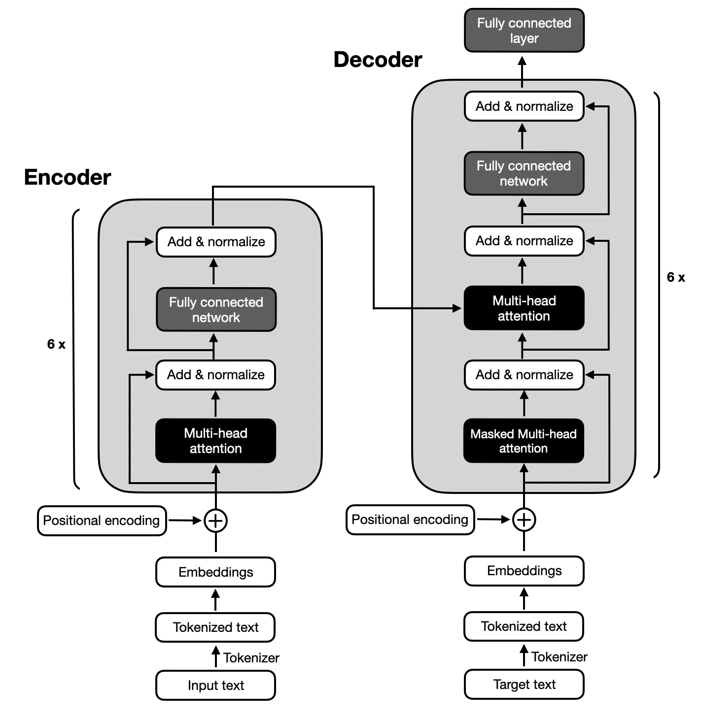
At the core of the Transformer is the attention mechanism, specifically multi-head attention. This allows the model to create rich contextual representations of a token's meaning by integrating information from surrounding tokens, effectively capturing relationships over long distances.
1. Attention
1.1. Self-attention
Attention is a mechanism used in transformers to help a model focus on relevant parts of the input sequence when creating representations for each token. Instead of processing each token independently, attention allows the model to weigh and combine information from other tokens in the sequence. This process helps the model capture relationships between tokens and build better context-aware representations.
In a transformer, attention works by taking the representation of a token at layer and computing how much each of the other tokens should contribute to the token’s new representation at layer . This is done by calculating attention scores, which reflect the relevance of each token to the one being processed.
Self-attention is a type of attention mechanism where each token in the sequence attends to (or "pays attention to") every other token, including itself. This allows the model to capture dependencies between tokens, regardless of their position in the sequence.
In self-attention, each token in the sequence is represented by three different types of vectors that capture distinct roles during the attention process. These roles are query, key, and value, and each token plays one of these roles at any given time.
To compute self-attention, transformers introduce three sets of weight matrices: , , and . These weight matrices are used to transform the input token representation into the query, key, and value vectors.
- Query vector is used to compute the attention scores with other tokens to determine which ones are most relevant to the current token.
- The key vector helps to measure the similarity between tokens, allowing the model to decide how much attention to give each token based on the query-key comparison.
- The value vector contains the information (or "value") that will be aggregated and passed to the next layer
The self-attention mechanism computes attention scores by comparing the query vector of the current token with the key vectors of the previous tokens, then using these scores to weight the value vectors of those tokens. The weighted sum of the value vectors becomes the output for the current token.
To calculate the attention scores , which determine how much focus one token should have on another, we first compute the dot product between the query vector of the current token and the key vector of the other token :
However, the raw dot product can result in large values, especially as the model dimensionality increases, which could lead to gradient instability during training. To mitigate this, we scale the dot product by the square root of the dimensionality of the key vectors, , which helps maintain stable gradients:
After computing the attention scores, we use them to weight the value vectors of all tokens. The final output for a token , denoted as , is the weighted sum of the value vectors, where the weights are the attention scores:
This output, , represents the context-aware embedding of token , combining information from other tokens in the sequence, weighted by how relevant each token is to .
1.2. Multi-head attention
Multi-head attention is a mechanism within transformers that extends self-attention by allowing the model to attend to different aspects of the input simultaneously. This is achieved by using multiple attention heads, each operating independently but in parallel.
- One for syntactic relatedness
- One for semantic relatedness
- One for coreference, etc
In multi-head attention, the attention mechanism is applied multiple times in parallel, with each attention "head" using its own set of learned parameters. Each head independently computes attention using its own query, key, and value matrices:
- Query vector:
- Key vector:
- Value vector:
For each head , the attention scores are computed as:
Concatenate all head vectors and project then
2. Position embeddings
Self-attention mechanisms in transformers do not inherently capture the order of words in a sequence. This lack of positional information can be problematic because the meaning of a sentence often depends on the order of its words.
To address this, transformers use position embeddings to encode the position of each token in the sequence. These embeddings are then added to the token embeddings, allowing the model to incorporate both the semantic meaning of the words and their positions in the sequence.
Simple solution: Concatenate the semantic word embedding with an absolute position embedding. This combined embedding is then used as the input to the transformer model, enabling it to understand the order of words in addition to their meanings.
Multi-head self-attention isn’t quite sufficient. We need a few extra things and package everything up into so-called Transformer blocks.
3. Types of Transformer models
4.1. Sequence Encoders with self-attention
Encoder self-attention covers the entire sequence, i.e. both the words to the left of the current position and the words to the right of the current position.
Text classification (one label per sentence)
- Train a model on the MLM task, adding a
[CLS]token in front of every sentence - Throw away the output layer, create a new one
- Fine-tune the model to predict the label at the
[CLS]position
- Train a model on the MLM task, adding a
Sequence labeling
- Train a model on the MLM task
- Throw away the output layer, create a new one
- Fine-tune the model on POS-annotated data
4.2. Sequence Decoders with self-attention
- Attention can only access tokens to the left.
- But typically, far-way tokens get less attention.
- Decoder self-attention only covers the words to the left of the current position (because the words to the right are not yet known at test time).
4.3. Encoder-Decoder model with cross-attention (Machine Translation)
- Train an Encoder for the Source Language: The encoder processes the input sequence in the source language and generates a set of context-aware representations for each token.
- Train a Decoder for the Target Language: The decoder generates the output sequence in the target language, using the context provided by the encoder.
- Connecting Encoder and Decoder:
- First Idea: Directly connecting the encoder and decoder can work if the source and target languages have the same word order.
- Cross-Attention: To handle different word orders and improve translation quality, we use cross-attention. Cross-attention allows the decoder to focus on relevant parts of the source sequence by attending to the encoder's output representations.
II. Large Language Models (LLMs)
1. Definition
LLMs are advanced machine learning models designed to predict the next word in a text sequence. These models leverage deep neural networks based on the Transformer architecture and contain billions of parameters. They are trained on vast amounts of text data collected from the web.
- Key Mechanism: Self-Attention
- Input: A sequence of tokens.
- Output: Probabilities for the next token.
Self-attention allows the model to weigh the importance of different tokens in the sequence, enabling it to capture contextual relationships and dependencies between words, regardless of their distance from each other in the text.
2. Training Process
The LLM is trained through self-supervision:
Given a text made of tokens , we take partial sequences and seek to predict the next token .
The LLM will take as input and output a probability distribution over possible next tokens.
The loss for this token is then defined as the cross-entropy:
- Explanation: Probability of the actual token in the output distribution .
We then make (at batch level) a small update on the model weights to reduce the loss.
Basic model update through stochastic gradient descent (SGD):
- Explanation:
- : Current model weights.
- : Gradient of the cross-entropy loss as a function of the model weights.
- : Learning rate (controls the step size of each update).
- Explanation:
LLM training relies on optimizers that are variants of SGD:
- Such as Adam (Adaptive Moment Estimation).
- Distributed training setup using many GPUs.
3. Dominant LLMs Architectures
Encoder-Only
For these models, attention layers can access all the words in the input sentence, allowing the model to process the entire sequence simultaneously and encode it into a comprehensive context vector. This type of model is well-suited for tasks that require an understanding of the full sequence, such as sentence classification, named entity recognition, and question answering.
A prominent example of an encoder-only model is BERT (Bidirectional Encoder Representations from Transformers), proposed in 2018. BERT is pre-trained on a large corpus of text using two primary tasks: masked language modeling (MLM) and next-sentence prediction (NSP).
- Masked Language Model (MLM): specific words in a sentence are randomly masked, and the model learns to predict these missing words based on the context provided by the remaining words.
- Next Sentence Prediction (NSP): helps BERT determine whether a sentence is contextually related to the preceding sentence. This allows BERT to better understand the relationships between sentences and the context of each individual sentence.
Other techniques, such as Word2Vec, FastText, and GloVe, generate word representations based on their common contexts. However, the contexts in natural data can be diverse. While models like Word2Vec and FastText produce a single vector representation for each word derived from a large dataset, they do not capture the richness of different contexts. In contrast, creating representations of each word based on the other words in the sentence yields more meaningful results. BERT improves upon earlier methods by generating context-dependent representations that take into account words both before and after a target word, resulting in a language model with richer semantics.
Decoder-Only
For these models, attention layers can only access tokens to the left of the current position, leading to a focus primarily on preceding words. Consequently, tokens that are further away receive less attention. These models are often referred to as auto-regressive models because their pretraining is typically formulated around the task of predicting the next word (or token) in a sequence. Decoder-only architectures excel in tasks involving text generation, making them a key focus in the development of large language models (LLMs) today.
These models are trained in an unsupervised manner on vast amounts of unlabeled data, and their architecture has been optimized as model sizes have scaled significantly. GPT (Generative Pre-trained Transformer) models are prominent examples of this model category.
Encoder-Decoder
For these models, the attention layers of the encoder can access all words in the initial input sentence, while the attention layers of the decoder only consider the words that precede a given word in the output sequence. These models are typically pretrained using the objectives suitable for either the encoder or the decoder, enabling them to perform both understanding and text generation tasks.
However, several factors contribute to the relative infrequency of scaling encoder-decoder architectures into large language models (LLMs):
- Training Complexity: Training a model with an encoder-decoder architecture requires data to be in the form of input-output pairs, which makes the preparation of training data quite costly and time-consuming. The need for paired data can limit the availability of suitable datasets for certain tasks. The encoder-decoder model operates in two steps. In contrast, encoder-only or decoder-only models can perform inference in a single step, which simplifies the process and can lead to quicker generation times.
- Task Specificity: The encoder-decoder architecture is specifically designed for certain tasks, such as machine translation, where there is a clear correspondence between input sentences and output sentences. In contrast, the goal of LLMs is to handle a wide variety of generative tasks like text completion and question-answering. LLMs need to be flexible enough to adapt to different types of prompts and generate coherent text without supervision.
Quick Recap
- Encoder-only
Masked language modeling: Predicts masked tokens in a sentence.
Smaller & older models: Still effective for information extraction tasks.
- Decoder-only
Dominant LLM approach: Auto-regressive next-token generation.
- Encoder-decoder
Self- & cross-attention: Combines both for input→output mapping.
Machine translation & structured tasks: Suited for paired input-output data.
4. Model Alignment
4.1. Fine-tuning
Once a model has been pre-trained, it can be fine-tuned for a specific task. Fine-tuning involves additional training with smaller amounts of in-domain data, using the pre-trained model as a starting point. This process is much more data-efficient than training a model from scratch because the pre-trained model has already learned useful semantic representations that can be transferred to the new task.
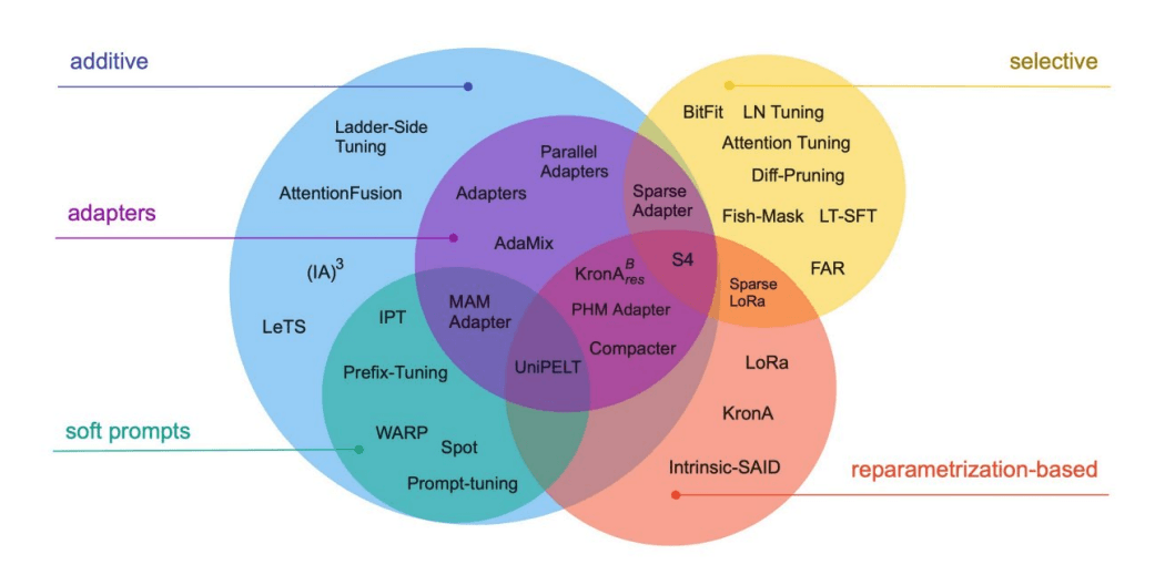
During fine-tuning, only a small fraction of the parameters are optimized, a technique known as Parameter-efficient Fine-tuning (PEFT). PEFT techniques include:
- Adapters: These are small trainable modules inserted between layers of the pre-trained model. Adapters allow the model to learn task-specific adjustments without modifying the original model parameters extensively.
- LoRA (Low-Rank Adaptation): This technique modifies the model weights using low-rank matrices. By decomposing the weight updates into low-rank matrices, LoRA reduces the number of parameters that need to be trained, making the fine-tuning process more efficient.
- Soft Prompting: In this approach, trainable vectors are appended to the input prompt. These vectors are optimized during fine-tuning to guide the model's responses towards the desired task-specific outputs.
- IA3 (Intrinsic Attention-guided Adaptation): This method adjusts the attention mechanism in transformer layers. By fine-tuning the attention weights, IA3 allows the model to focus on task-relevant parts of the input sequence, improving performance on the specific task.
These PEFT techniques enable efficient adaptation of large pre-trained models to new tasks with minimal computational resources and data requirements.
4.2. Two Alignment Strategies
Instruction Tuning: This involves training the model to follow specific instructions by providing it with pairs of instructions and correct responses.
- Manually: Humans write questions or problems and their correct answers.
- Dataset Conversion: Existing datasets for supervised NLP tasks (e.g., text classification, sentiment analysis, NER, machine translation) are converted into instruction-response pairs.
- LLM Generation: Large language models generate instruction-response pairs based on external databases and general guidelines.
Preference Alignment: This involves aligning the model's responses with human preferences using preference data, such as ratings of answers to prompts.
- Common Format: Triples of the form
<prompt, chosen response, reject response>. - Data Collection: Ratings can be collected by paying crowdworkers (following guidelines on what constitutes a “good” response) or by asking users to rate the responses they receive.
- Common Format: Triples of the form
5. Prompting
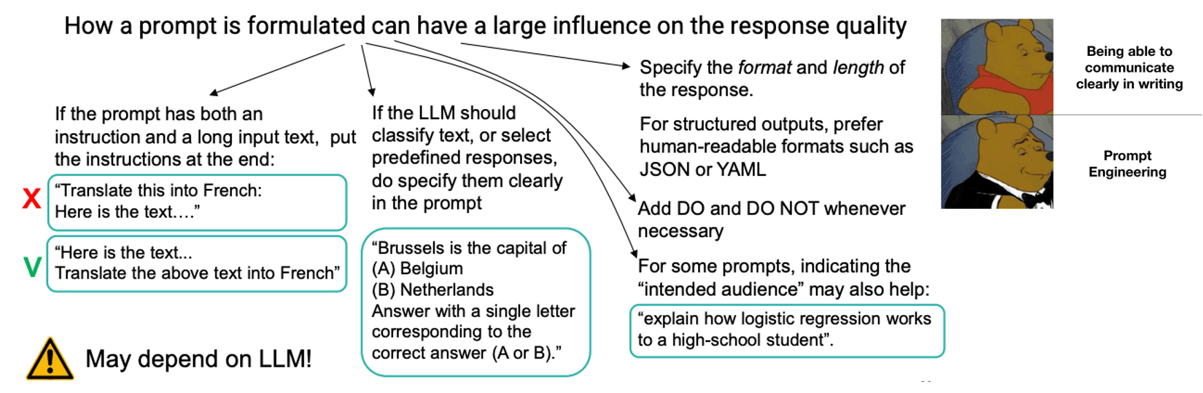
A prompt = input to the LLM, which can be a question or instructions on the task to perform.
- System prompt: Generic instructions, defined by the system provider, on how the system should respond (be helpful, avoid offensive language, etc.) and how it should present itself to the user (“You are ChatGPT, a large language model trained by OpenAI…”)
- User prompt: Specific instructions provided by the user.
5.1. In-context Learning
In-context learning, also known as few-shot prompting, involves providing the model with a few examples or demonstrations within the prompt to help it understand the desired output for a given task. This technique is particularly useful for complex tasks where the model might need additional context to generate accurate and relevant responses.
By including examples in the prompt, the model can learn from these instances and apply the learned patterns to produce the expected output.
5.2. Chain-of-Thought
But those “reasoning” capabilities can be improved by forcing the LLM to generate longer, step-by-step responses
- “Let’s think step by step”
- In-context demonstrations of reasoning steps involved in solving similar problems
- Can also ask the model to criticize or debate its own responses
6. Generation
Assume we have a trained a generative LLM that takes as input a list of and return a probability distribution over the next token
6.1. Greedy Decoding
- At each step, just select the token with highest probability
- And continue until a special
<eos>token, or the maximum output length
But greedy decoding is short-sighted ↔ Can get trapped in local minima (good “local” choice of token, but poor text at the end, with no way to backtrack)
6.2 Beam search decoding
- We keep at each step a "beam" of K hypotheses representing the best partial outputs so far
- Those K hypotheses are gradually expanded, token by token
- Until we reach
<eos>or the maximum output length - Finally, we take the hypothesis with max probability among the K alternatives
6.3. Top-K sampling
- At each step, we select the K tokens with highest probability
- We sample the next token only among those
Kpossibilities (after renormalising the distribution) - And continue until
<eo>or max sentence length
6.4. Top-p sampling
- Same principle, but instead of a fixed K, we select tokens among those making up the top
p%of the probability mass
6.5. Temperature
The creativity of the generation can be controlled by the temperature
- Temperatures < 1 will make the decoder more “conservative”, increasing its focus on high-probability tokens
- Temperatures > 1 will make the decoder more “creative” and sometimes select less-likely tokens
7. Retrieval-augmented generation
Retrieval-augmented generation (RAG) is a method to enhance LLMs by connecting them to external databases or specialized knowledge sources.
7.1. Shortcomings of LLMs
- Static Knowledge: Cannot add, remove, or update factual knowledge without retraining the model.
- Lack of Transparency: Difficult to inspect the model's knowledge or determine which source in the training data influenced the model's answers.
7.2. Basic Idea
- Retriever: Given a user prompt, search for relevant documents in a text database (Information Retrieval Task).
- Reader: Retrieve the most relevant texts and add them to the prompt to generate the response.
7.3. Advantages of RAG
- Easier to edit the LLM’s factual knowledge: simply update the underlying database, without needing to retrain the LLM!
- Cleaner distinction between "linguistic" and "factual" knowledge
- Better transparency: if a model produces a wrong answer, we can check whether the error stems from the retrieved documents
- Better attribution: the LLM can indicate the sources that have been used to generate its response
Reference
- Lecture 7 - NN2, IN4080, Autumn 2024, University of Oslo
- Lecture 8 - NN2, IN4080, Autumn 2024, University of Oslo
- Speech and Language Processing. Daniel Jurafsky & James H. Martin. Copyright © 2024. Draft of August 20, 2024. CHAPTER 9, The Transformer
- BERT: Pre-training of Deep Bidirectional Transformers for Language Understanding, Jacob Devlin, Ming-Wei Chang, Kenton Lee, Kristina Toutanova, 2018